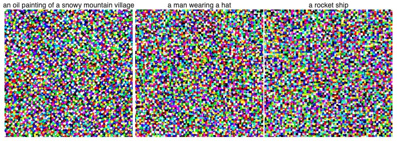
1 Inference Step
Name: Brandon Wong
The purpose of project 5A is to get familiar with the usage of diffusion models by implementing diffusion sampling loops and using them for other tasks such as inpainting and creating optical illusions. This was done using the stages 1 and 2 of the DeepFloydIF diffusion model. Before each time results were obtained, a seed was set. This part was done in Colab. The unet instance from stage 1 was used for most sections, although section 0 looked at examples with different numbers of inference steps.
This section was mainly just looking at results from the DeepFloydIF diffusion model as a point of comparison as an example of what is partially being implemented throughout the rest of this project. Results at 1 , 5, 10, 20, 40, and 100 inference steps (in stage 1) were observed, shown below. The seed used to ensure reproduceability was 714. Some results of adding different numbers of steps in stage 2 were also looked at (not shown), but as stage 2 is just upscaling from the results of stage 1 it really only affected image clearness and quality. Increasing the number of inference steps increased the general reasonables of the image, although improvements really started decreasing at around 10 steps. It was interesting to see how later steps moved in the direction of art rather than attempt to be realistic.

1 Inference Step
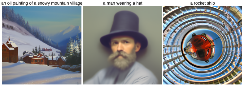
5 Inference Steps
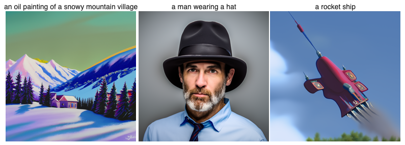
10 Inference Steps
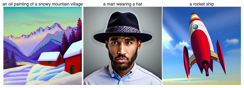
20 Inference Steps
40 Inference Steps
100 Inference Steps
In this section, I implemented a forwarding function to add noise at different timesteps based on the alpha values at different timesteps selected by the DeepFloydIF model. The equation to calculate x_t, the image at different timesteps, is shown below. Examples of an image with noise added at timesteps 250, 500, and 750 are also shown below alongside the original image without noise.
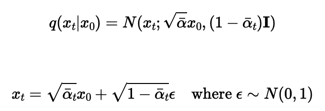
Forwarding Process Definition and Equivalent Equation

64x64 Image of the Campanile

Noise at Step 250

Noise at Step 500

Noise at Step 750
Once the forwarding results at the three timesteps were obtained, I used gaussian blur filtering to see what those results would look like, shown below.

Blur at Step 250

Blur at Step 500

Blur at Step 750
The use of a pretrained UNet model for denoising was also used to see what those results would look like if noise was reduced in one step.

UNet One Step at Step 250

UNet One Step at Step 500

UNet One Step at Step 750
In this section, I finally used iterative denoising (diffusion) with step skipping to speed it up. Starting at step 990, steps of size 30 were taken until step 0, the original image, was obtained after starting from a noisy image. In this specific section, the iteration started from the tenth timestep to ensure the resulting image was close to the original. The equations used to find the predicted previous image at each step is shown below.

Iterative Process Equation
This process was run on a noisy campanile image. The resulting images at every fifth timestep are shown below. The original image, resulting image, UNet result, and gaussian blur result are all also shown below.
.png)
Iterative Prediction at Step 90
.png)
Iterative Prediction at Step 240
.png)
Iterative Prediction at Step 390
.png)
Iterative Prediction at Step 540
.png)
Iterative Prediction at Step 690

Noisy Image

Iterative Result

One Step Result

Gaussian Blur Result
Instead of starting from the tenth timestep, this time the iterative process was started from the first one with a completely random image. This allowed for generation of completely new images, with the prompt used being "a high quality image" for the input to the model at each step.

Random Image 0

Random Image 0

Random Image 0

Random Image 0

Random Image 0
To improve the images, classifier free guidance was added to the iterative denoiser by computing the estimated noise both conditioned on a text prompt and unconditional. The overall noise estimate is the unconditional estimate plus a scale factor multiplied by the difference between the estimation on a prompt and the unconditional estimate. Five examples the the result of this are shown below. A scale factor of 7 was used with the prompt being "a high quality photo" each time.

CFG Random Image 0

CFG Random Image 0

CFG Random Image 0

CFG Random Image 0

CFG Random Image 0
Noise was added to images in varying amounts up to certain timesteps before running the CFG iterative denoising function on them to see what results would occur from denoising at certain points. This was done on three images; the campanile, a picture of a mug with cal on it, and a picture of a plushy. These results are shown below.

Campanile 1

Campanile 3

Campanile 5

Campanile 7

Campanile 10

Campanile 20

Campanile Original

Cal Mug 1

Cal Mug 3

Cal Mug 5

Cal Mug 7

Cal Mug 10

Cal Mug 20

Cal Mug Original

Plushy 1

Plushy 3

Plushy 5

Plushy 7

Plushy 10

Plushy 20

Plushy Original
The same process as the previous part was done in this part, except this time it was done on one image obtained from the web and two very simple badly done/very vague drawn images. The first drawn image was kinda meant to be a sailboat metal battleship and the second was supposed to be a starry sky. The web image is from here.

Web Image
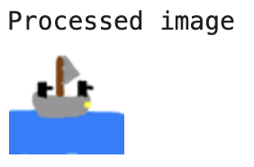
Drawn Image 1
Drawn Image 2

Web Image Results

Drawn Image 1 Results

Drawn Image 2 Results
By forcing the image at each step to have the forward prediction from the original image at all points that are not the mask, inpainting can be done, where only a select portion of the image develops a random result based on the image and the rest remain the original image. This is shown below on the campanile, mug, and plushy. The campanile ends up with a new top, the mug ends phased out of the image (a bit badly), and the plushy gets a nose.

Inpainting Process

Inpainted Campanile

Inpainted Mug

Inpainted Plushy
This runs the same thing as the first part of 7, but it runs guided by a prompt instead of nothing. This allows for interesting changes as the model attempts to obtain an image based on the prompt from the original image to varying extents as shown below on different stages of added noise on the campanile, mug, and plushy.

Prompt Based Translation from Campanile, Starting from Forwarding to Different Timesteps

Prompt Based Translation from Mug, Starting from Forwarding to Different Timesteps

Prompt Based Translation from Plushy, Starting from Forwarding to Different Timesteps
In this section, anagrams from two different prompts were developed. The noise from transforming an image from one prompt and the noise from transforming the flipped image from another promt were averaged for a combined transformation at each step until the final result appears to be one image right side up and another image upside down. This is shown below.

"an oil painting of people around a campfire" and "an oil painting of an old man"

"an oil painting of people around a campfire" and "an oil painting of an old man"

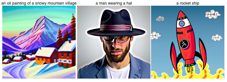
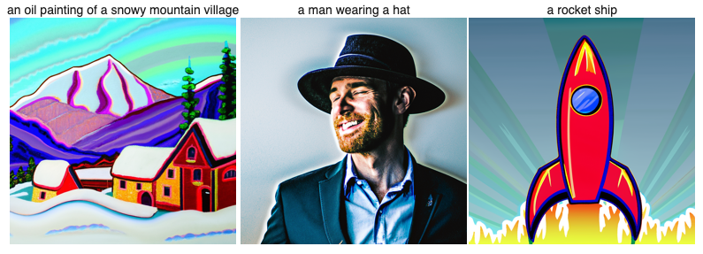
"an oil painting of a snowy mountain village" and "a photo of the amalfi cost"

"a rocket ship" and "a lithograph of waterfalls"
In this section, the low frequencies of the noise from running the model on the current step on one prompt and the high frequencies from running the model on the current step on another prompt were combined to form an overall noise to remove, which eventually reaches a hybrid image after all the iterations. A kernel size of 33 and a sigma of 2 was used. The results are shown below.

"a lithograph of a skull" and "a lithograph of waterfalls"

"a photo of the amalfi cost" and "a puffy cloud

"a space battleship" and "a chalk drawing of a skyscraper"
After having had fun working with with prebuilt models in Part A, in this part I implemented some basic versions of the model from the previous section. Three versions of UNet were made; single step, time conditional, and time and class conditional. Each was was an improvement from the previous one, built using pytorch to be able to at dirst denoise and then generate results from and based on the MNIST dataset. The first step was to make a noise generator function to train the models to denoise, with the results at different σ values shown below. Everything was done in Google Colab.
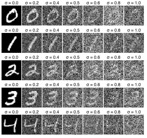
Noise at Different σ Values
The purpose of section 1 was to implement a basic version of UNet that could be used to try to denoise images in a single step, the simplest form possible.
To implement UNet myself, using the nn.Module class from pytorch, I first made classes for basic blocks that I then put together in a class for the UNet model. The basic blocks generally consisted of a convolution of some sort followed by a batch norm and then gelu, although there were several blocks that used things such as average pool and concatentation instead as those are also part of UNet. The number of channels in each section were generally some multiple of a hidden dimension hyperparameter.
After establishing a UNet model, I trained it on the MNIST training set. This was done over five epochs with batches of 256 images at a time. L2 loss, also known as the mean square error, was used to train the model. The model was trained on images noised with a σ of 0.5. The Adam optimizer was used to optimize the model with a learning rate of 1e-4. The hidden dimension for this model was set to 128. Overall, it took around 8 minutes with a final loss of 0.008393 on the last batch of data. After obtaining the trained model, testing was done to see how effective it would be on images with varying levels of noise added.
The results of the model are shown below. The loss over each step is the first image, and the only graph, shown below. The loss curve in the first epoch and fifth epoch are also shown to compare to each other. After that, the samples used for testing and observing the differences in effectiveness between training on one epoch and another epoch are shown, followed by the results at those two epochs. Finally the out-of-distribution results, where the model was testing on images noised with values other than 0.5 are shown beneath, with artifacts showing up significantly starting around σ = 0.8.
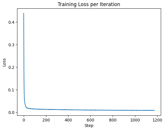
Plot of Loss per Step for UNet
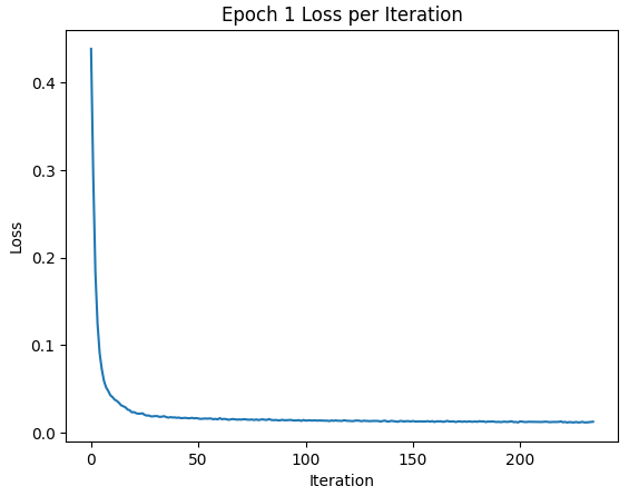
Plot of Loss per Step for Epoch 1
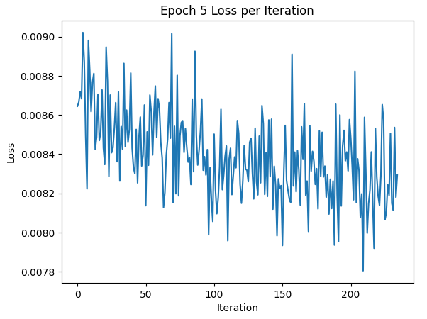
Plot of Loss per Step for Epoch 5
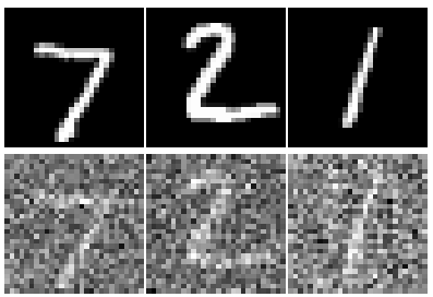
Samples for Testing
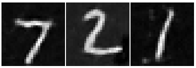
UNet Results at Epoch 1
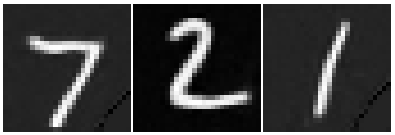
UNet Results at Epoch 5

Out-Of-Distribution Results 1

Out-Of-Distribution Results 2

Out-Of-Distribution Results 3
In this part, time conditioning and then classifier conditioning are both added to the UNet model put together previously to turn it from just a denoiser to a diffusion model, giving it the ability to iteratively denoise an image such that it can even generate new images from noise. This can be done using a combination of the equations used to put together the iterative denoiser in Part A and L2 loss on predicted noise, rather than the resulting image, generated by the UNet model from the first section with some additional fully connected blocks at specific parts to enable the model to take in a time and later classifier as inputs to the model. The β value for the chosen 300 timesteps range from 0.0001 to 0.02 evenly spaced apart, and the α values are the cumulative product of 1 minus the β values up to the timestep of each one.
To add time conditioning to UNet, fully connected blocks, which are just a linear function followed by a gelu function run on a timestep t, were added to the unflatten result and first upblock result. This allowed the model to account and adjust for the timestep whend deciding how much and what sort of noise there is. the fully connected blocks are run on a normalized t value to maximize effectiveness.
To train the UNet, a training algorithms is run using equations from Part A to calculate the resulting noise values at different timesteps. A batch size of 128 and 20 epochs were used to maximize the effectiveness of the new UNet. A hidden dimension of 64 was selected. The Adam optimizer was used with an initial learning rate of 1e-3, and a scheduler with a learning rate decay of 0.1 ^ 1/num_epochs. The loss to steps curve is shown below, with almost all the improvement at the beginning and everything after being quite gradual.
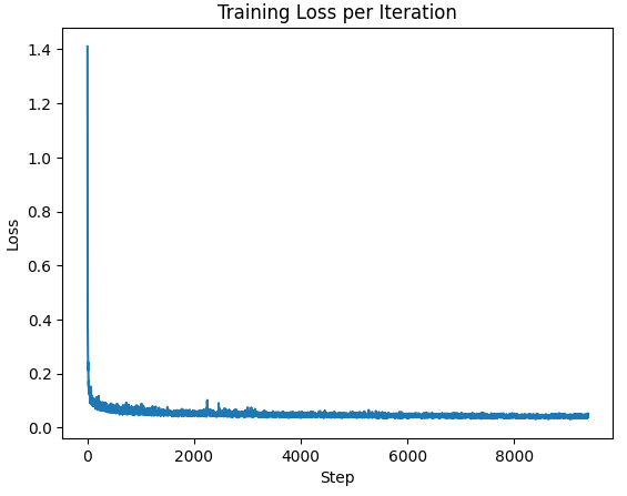
Plot of Loss per Step for Time Conditioning
Another algorithm was needed to properly sample the model, based on the iterative denoiser of Part A. The results of this model allowed for both the cleaning up of noisy images, including from a separate test set, and generation of new ones close to the original MNIST dataset. Examples of generating new images at epoch 5 and epoch 20 are shown below. The results of epoch 20 are slightly improved from the results of epoch 5, which makes sense as improvements became significantly more incremental after the first couple of epochs.

Time-Conditioned UNet at Epoch 5

Time-Conditioned UNet at Epoch 20
To complete the basic diffusion model, I added classifier based conditioning by ensuring the model could take a class as an input then use a one hot encoded result as an input to the fully connected block which would then be multiplies with the unflatten and upblock results before the time gets added to them. During training, the model is also set to ignore the classifier a tenth of the time. The classifier is set up to take ten classes, the digits from 0 to 9, due to it being the MNIST set. The training algorithm is just slightly modified from the time conditioning model to take in the class on top of the image and timestep. The loss of this model is shown below.
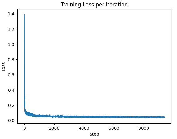
Plot of Loss per Step for Class Conditioning
One notable thing about using classifier based guidance is that on its own it is not very good (seen in Part A). As such, the unconditional noise predictions are needed as part of the sampling portion to ensure good results as seen in Part A. The γ value for this was set to 5.0. The results of the addition of class conditioned guidance is shown below for epoch 5 and epoch 20. The differences are less stark than in previous examples, but the epoch 5 results are generally a bit thicker and one of them has a leftover artifact, just standing out on its own.
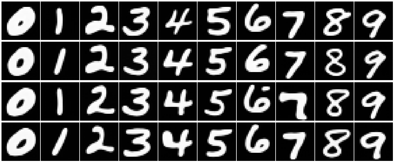
Class-Conditioned UNet at Epoch 5
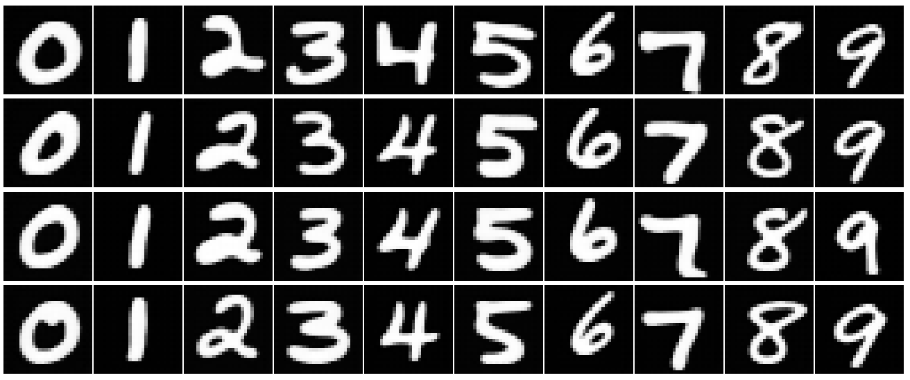
Class-Conditioned UNet at Epoch 20