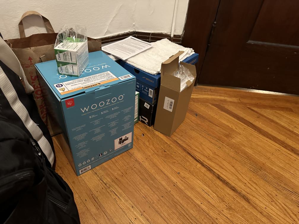
Box
Name: Brandon Wong
The goal of Project 4a is to warp images so that they can be stiched together into a single larger image with a single perspective. The first results of this part uses the described methods to rectify images, essentially converting images so that a part that should be a rectangle is displayed as one, warping the entire images so that it looks like its from the right perspective to see the rectangle as one correctly in the image. The second part warps images which are then manually aligned into a larger image.

Box
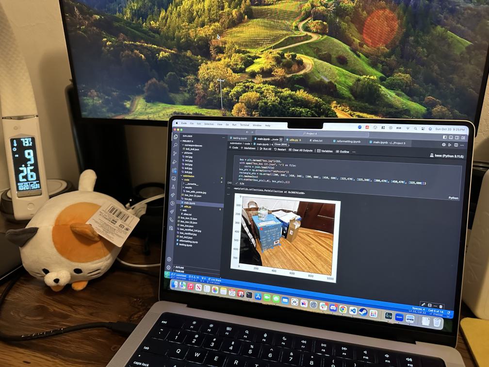
Computer
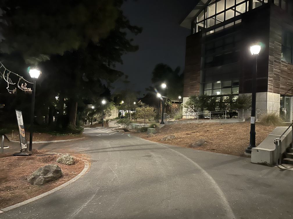
Path Left
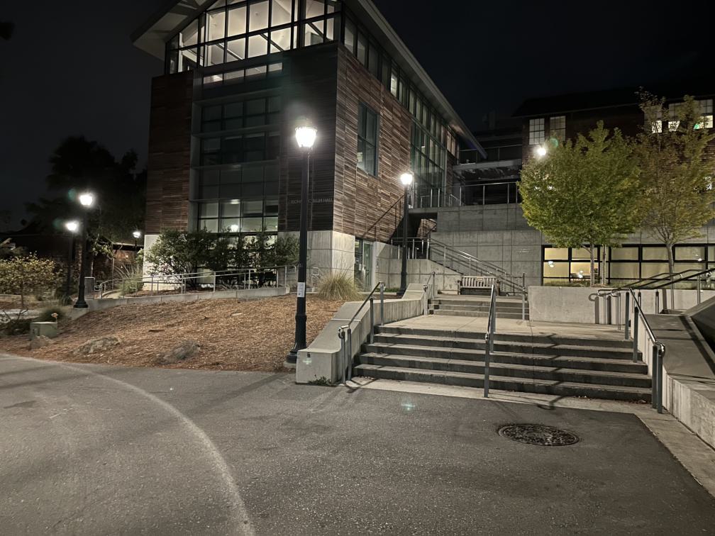
Path Right
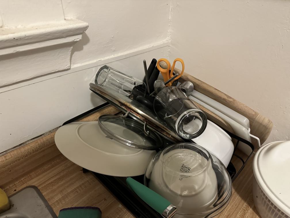
Dishrack Left
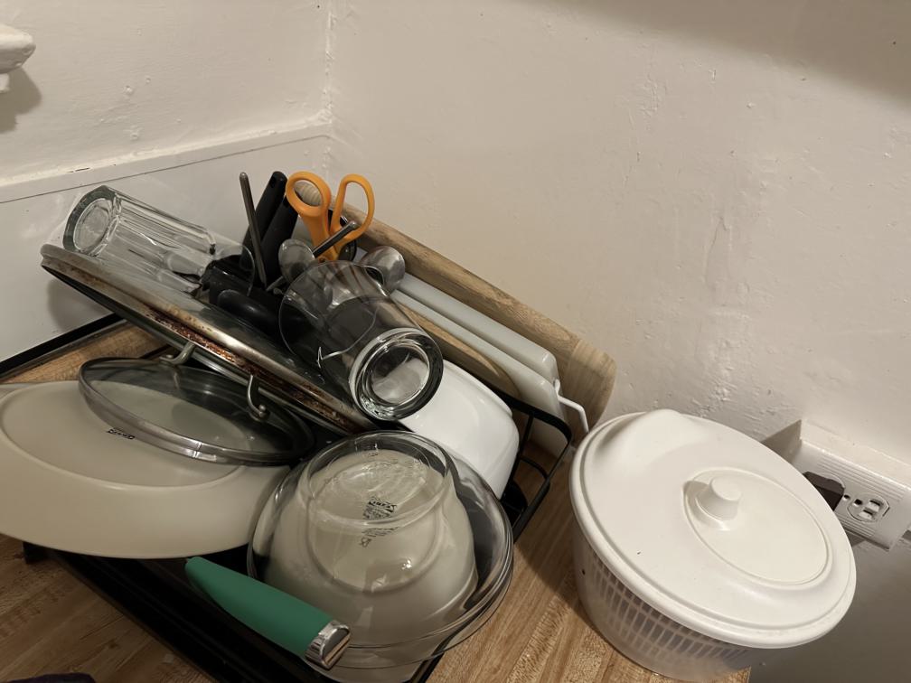
Dishrack Right
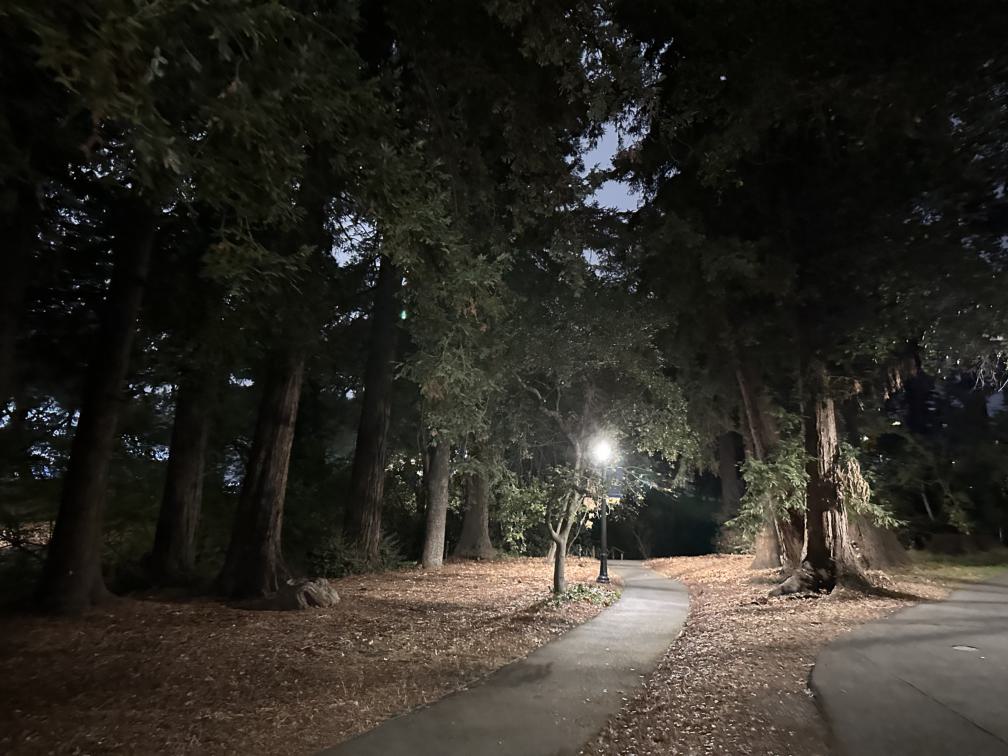
Split Path Left
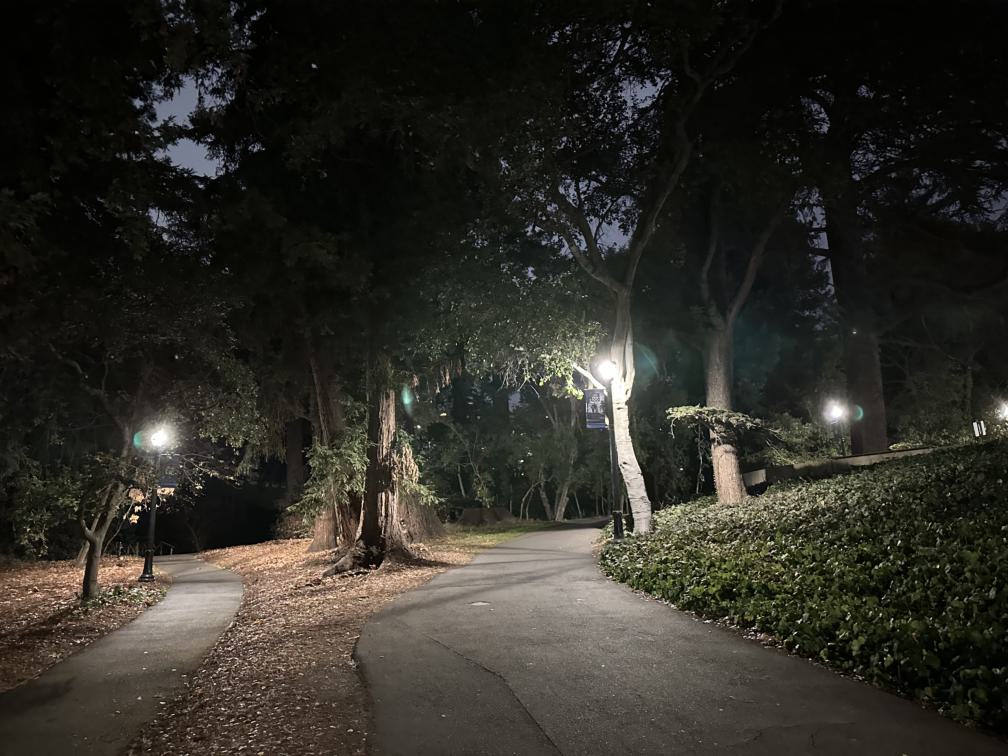
Split Path Right
To recover homographies, corresponding points were marked on the right and left images. For the images for rectification, the points that should be in a rectange were marked and than the rectanglular location of the points were manually input. This was done using the labeling tool given in the project spec linked here. Once the points were obtained, the homographies were computed using the least squared linear algebra function from numpy on the system of equations recovered from the matrix equation used to calculate homographies shown below. Inverse warping was then used by taking the inverse of the homography matrix and using that to calculate new warped images.
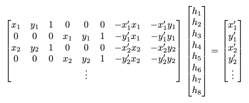
Homography Calculation Equation for Least Squares

Homography Equation Standard Form
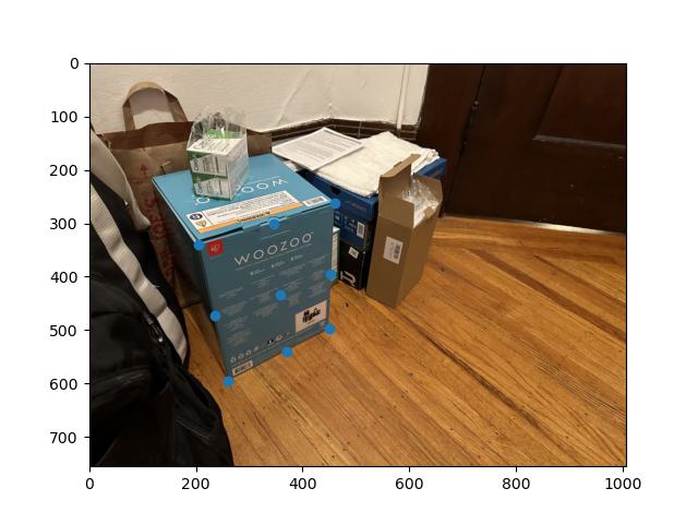
Box Points
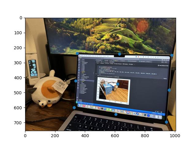
Computer Points
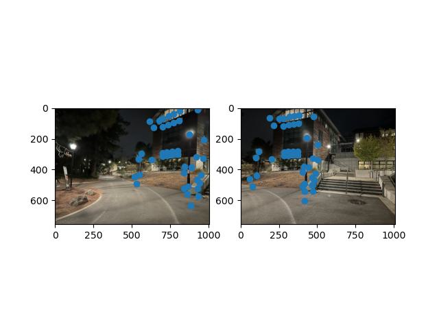
Path Points
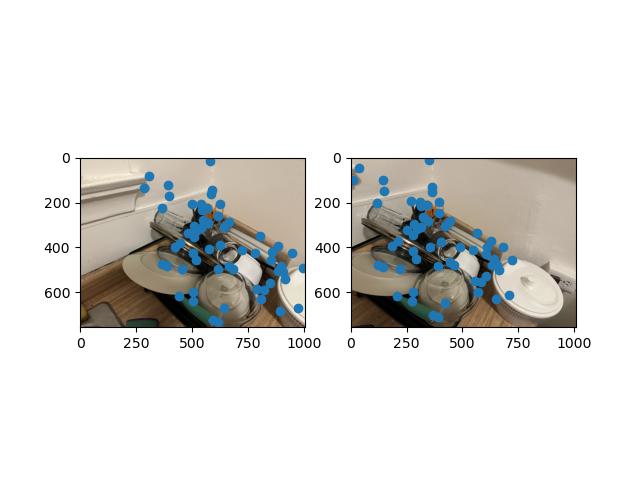
Dish Points
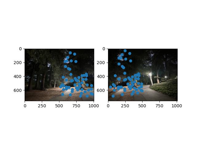
Split Path Points
To rectify images, the homography matrix for inverse warping was found, then the warp function made in the previous project was used to warp the old image into the new image with linear interpolation. There was a weird result where the box became super zoomed out due to stretching.
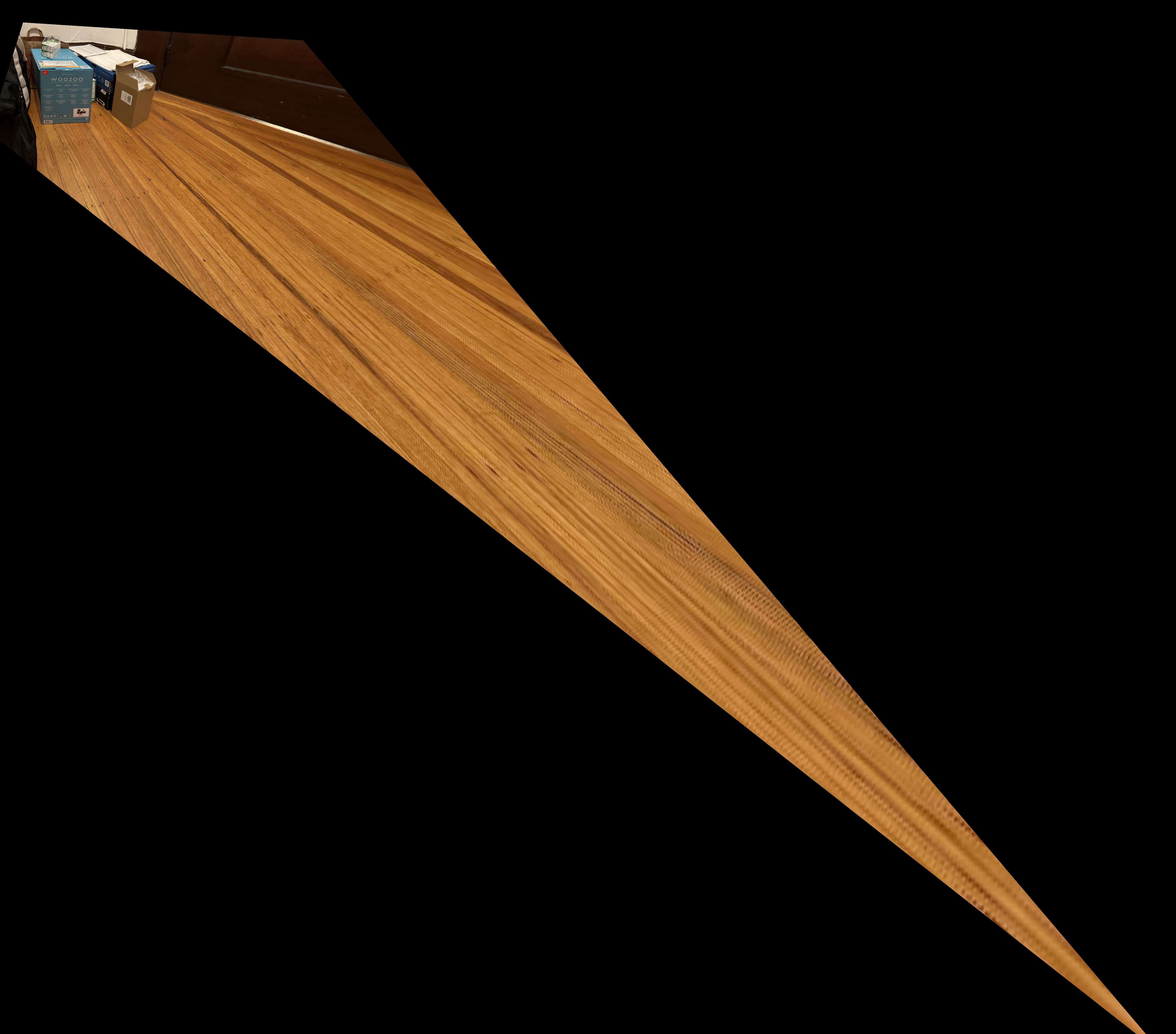
Box Rectified
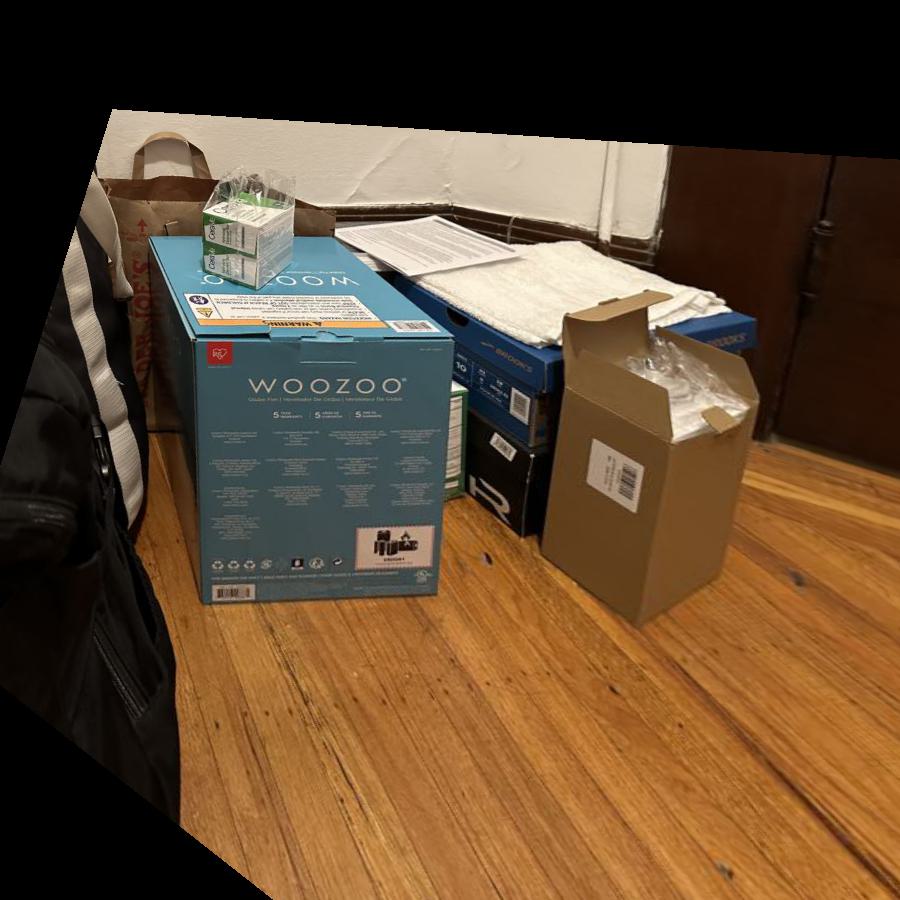
Box Rectified, Zoomed In
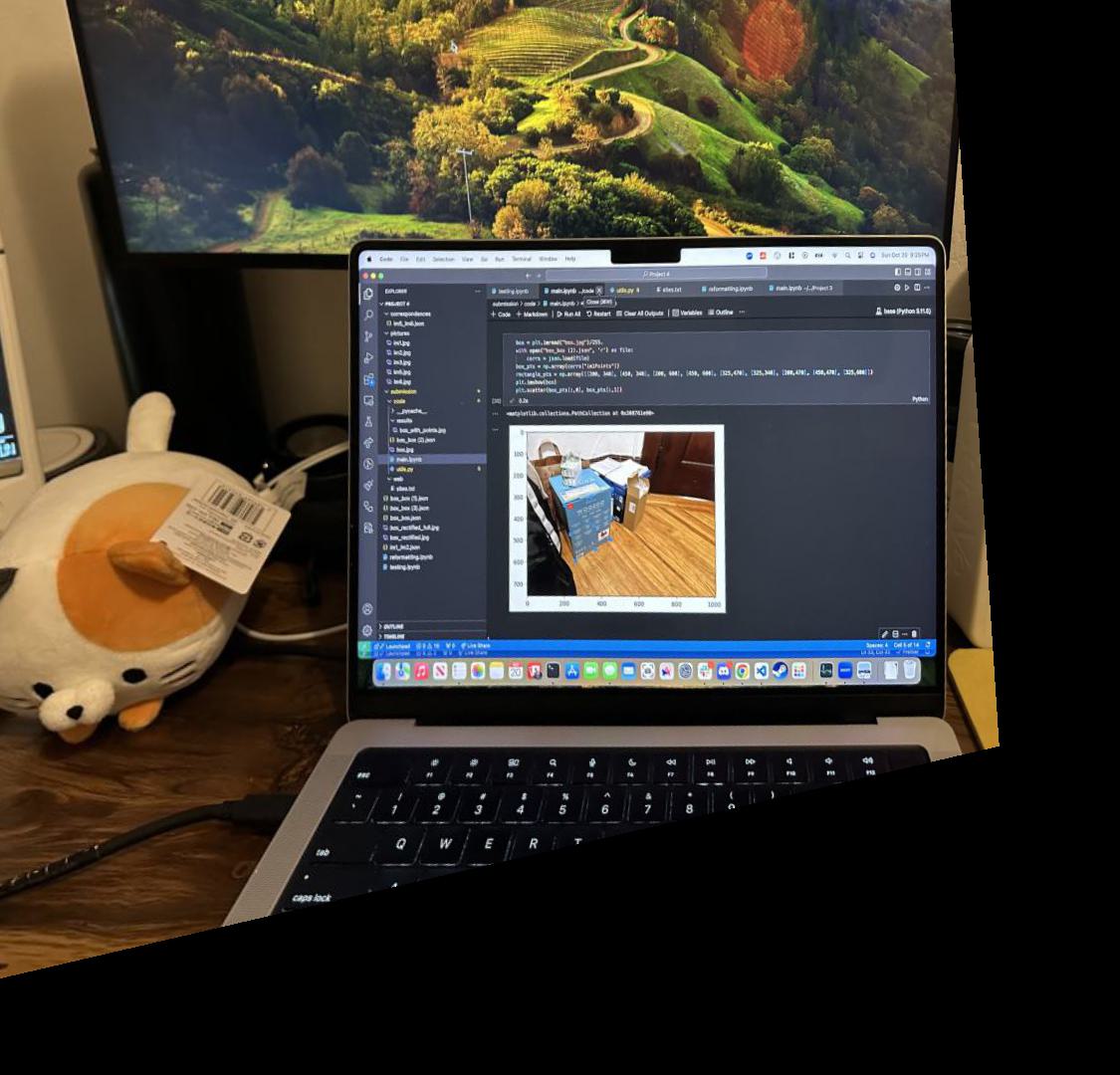
Computer Rectified
To create mosiacs, steps similar to the previous one were done. However, because the right side of the left image corresponds to the left side of the right image, the right corresponding points had to be shifted to ensure the full left image would be kept when warped. After that, the homographies could be calculated using those corresponding points. After that, the images could be put together onto a single larger image for a displayable combined result. To help remove some of the distinction between images as a result of differing brightness levels, multiresolution laplacian pyramid blending was used with the mask on the right image. The two images input were the warped left image and the combined image to prevent the black background on the rest of the image from causing issues in the blending. This helped slightly with the results.
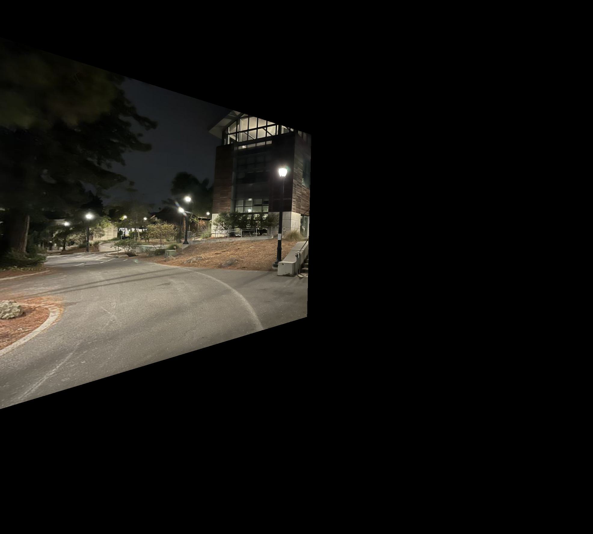
Path Left Warped
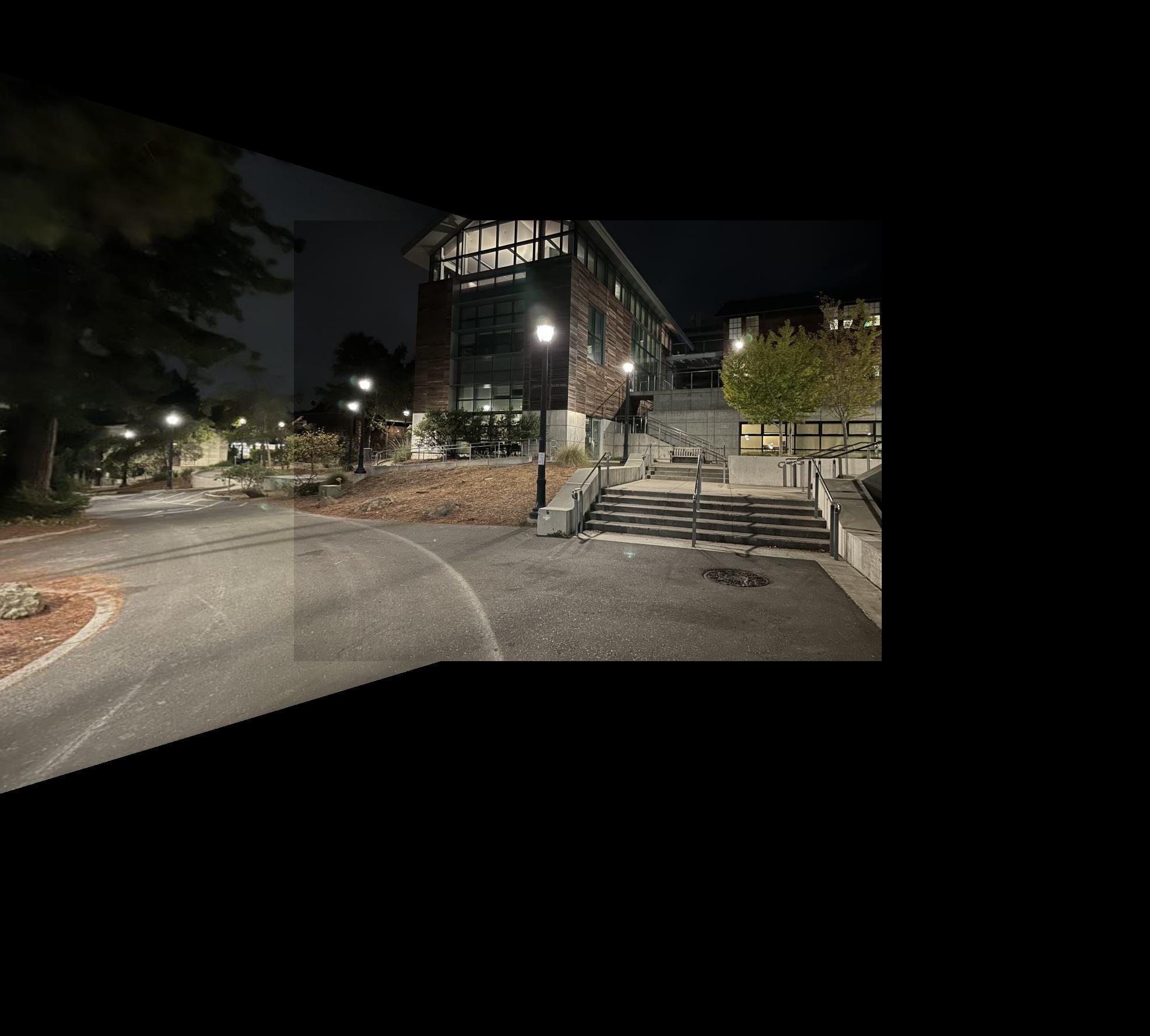
Path Mosiac, No Blending
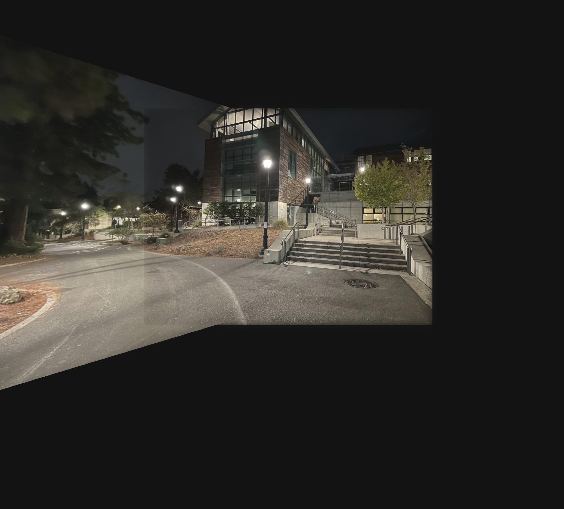
Blended Path Mosiac
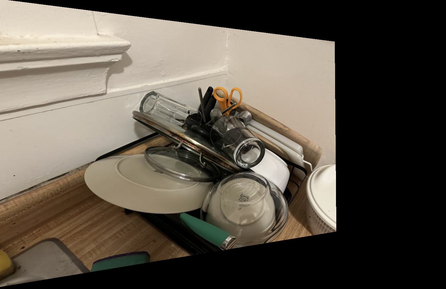
Dishrack Left Warped

Dishrack Mosiac, No Blending
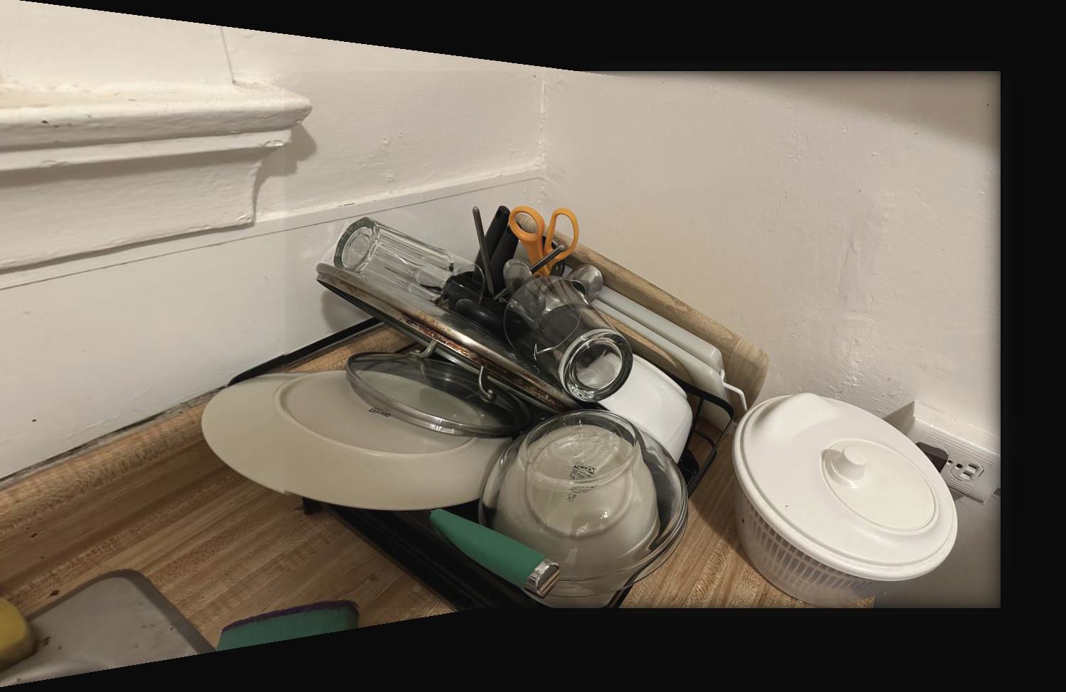
Dishrack Path Mosiac
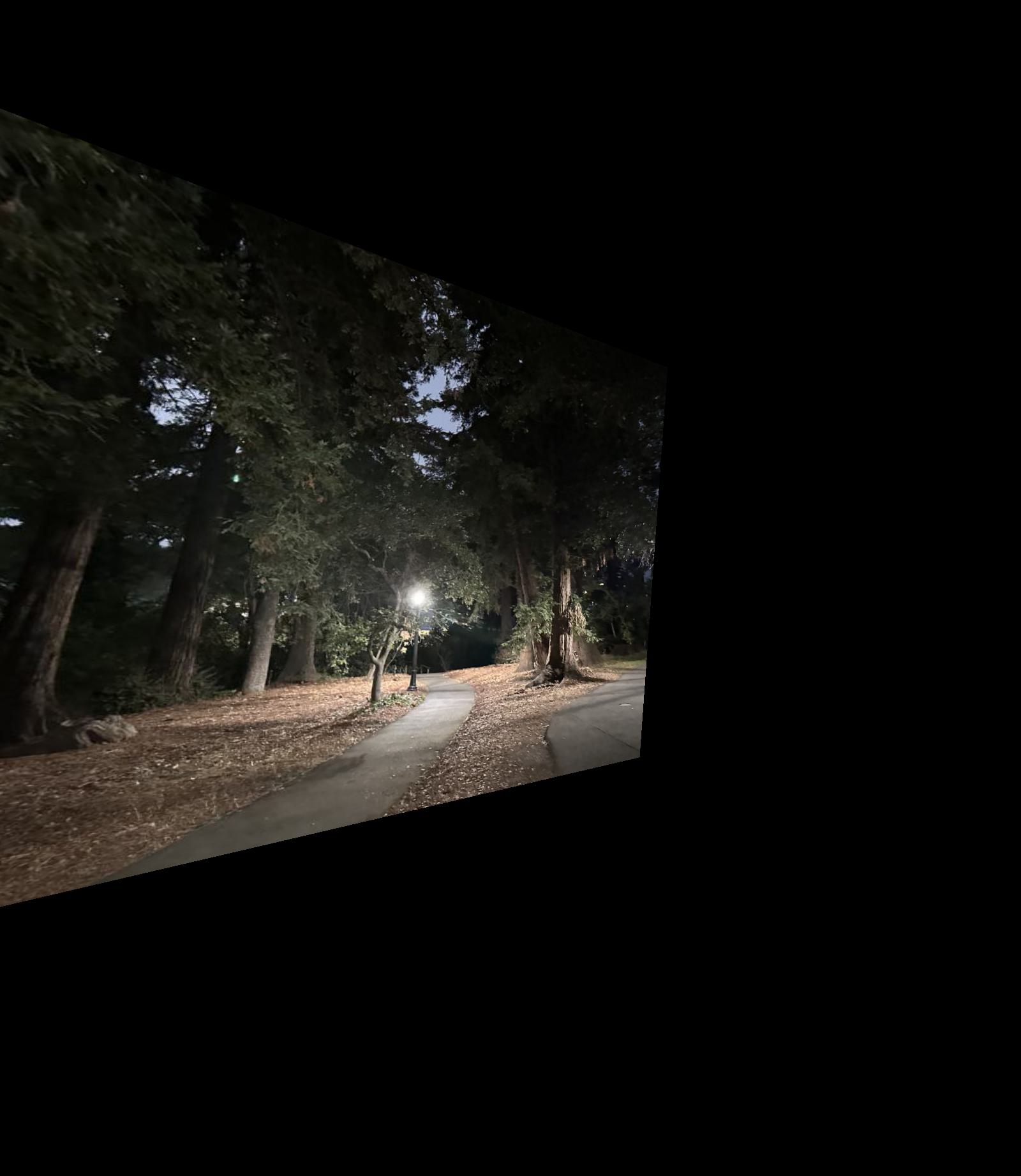
Split Path Left Warped
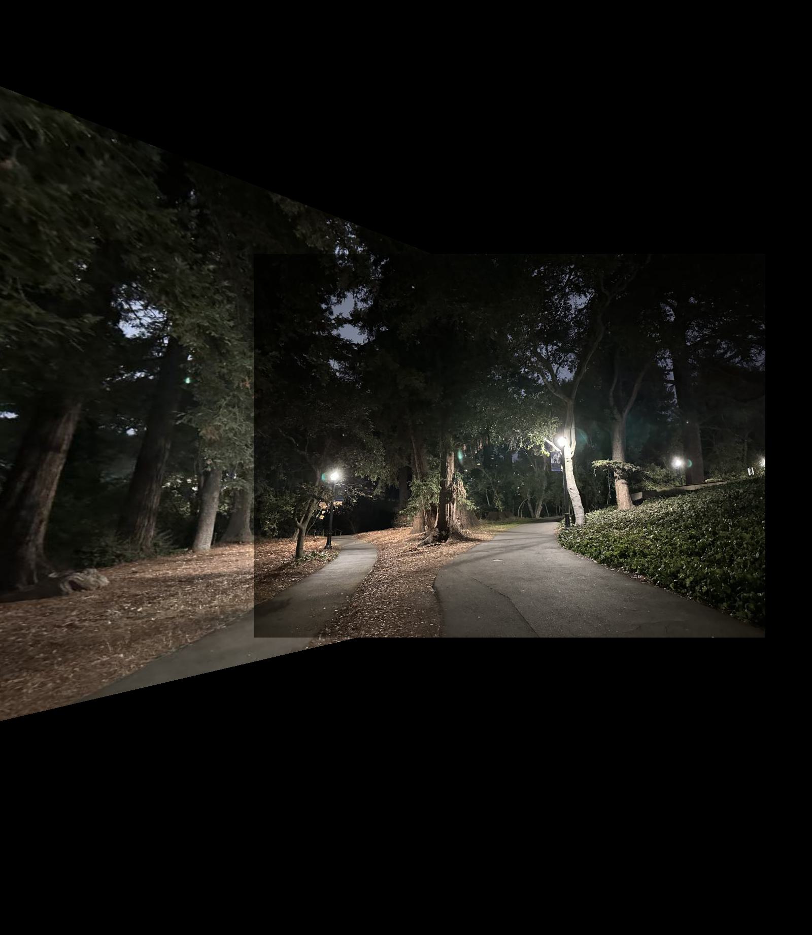
Split Path Mosiac, No Blending
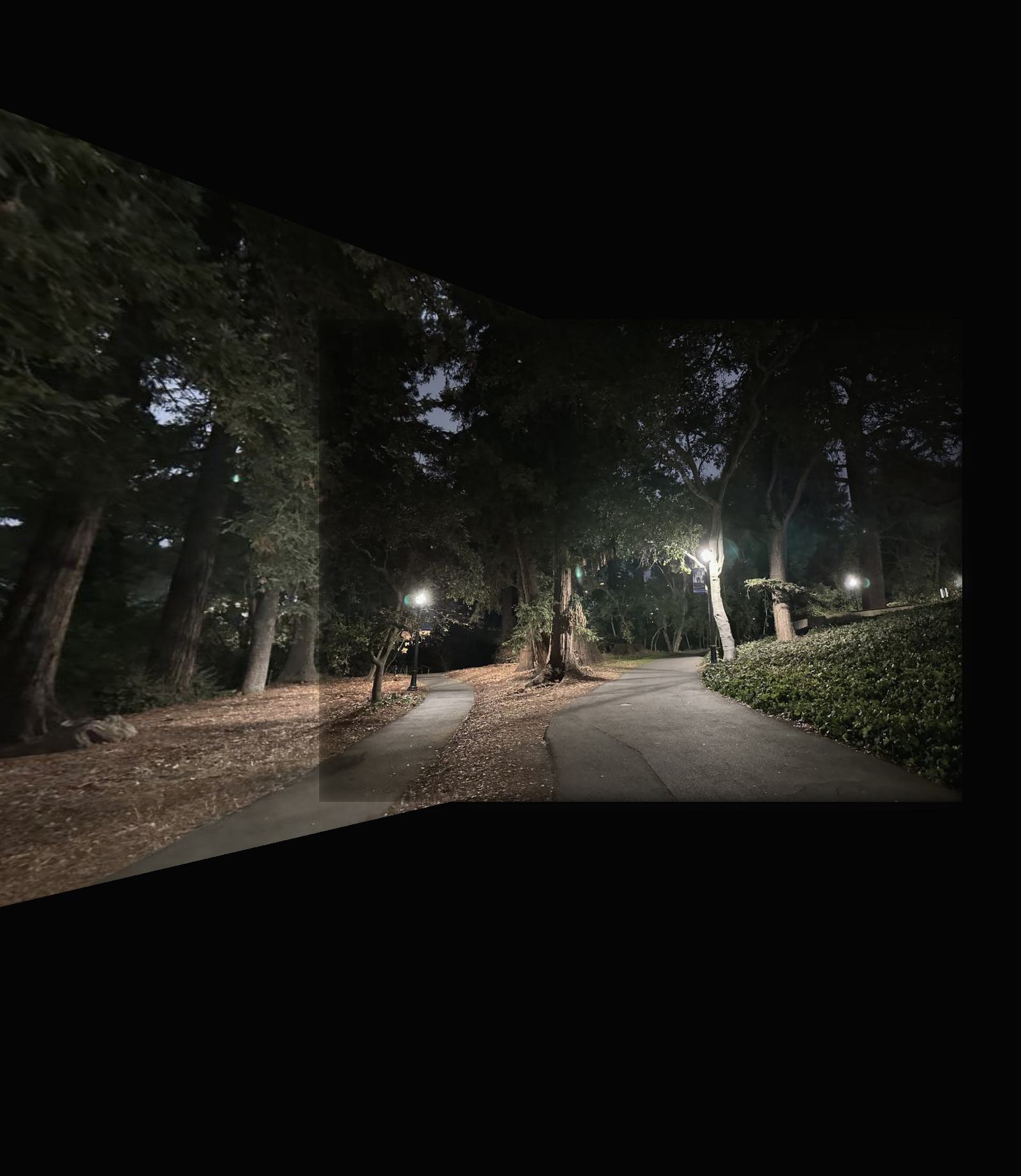
Split Path Mosiac
The goal of Project 4b is to find corresponding features in two images so they can be automatically warped and stitched together without requiring a human to select corresponding points between them. This is done through first using a Harris Interest Point Detector to find points of interest. Then, Adaptive Non-Maximal Suppression is used to select a balanced distribution of them, primarily the best ones. After this distribution is found, a descriptor is extracted for each feature, which is then used to match the features to the closest ones from the other image using Lowe's approach.
Interest points were detected via corner detection using the Harris corner detector. A space of 40 pixels was left empty on each side for use in the feature descriptor extraction later. The result was a very dense set of interest points that needed further processing to select the best ones to use as corresponding points between images.
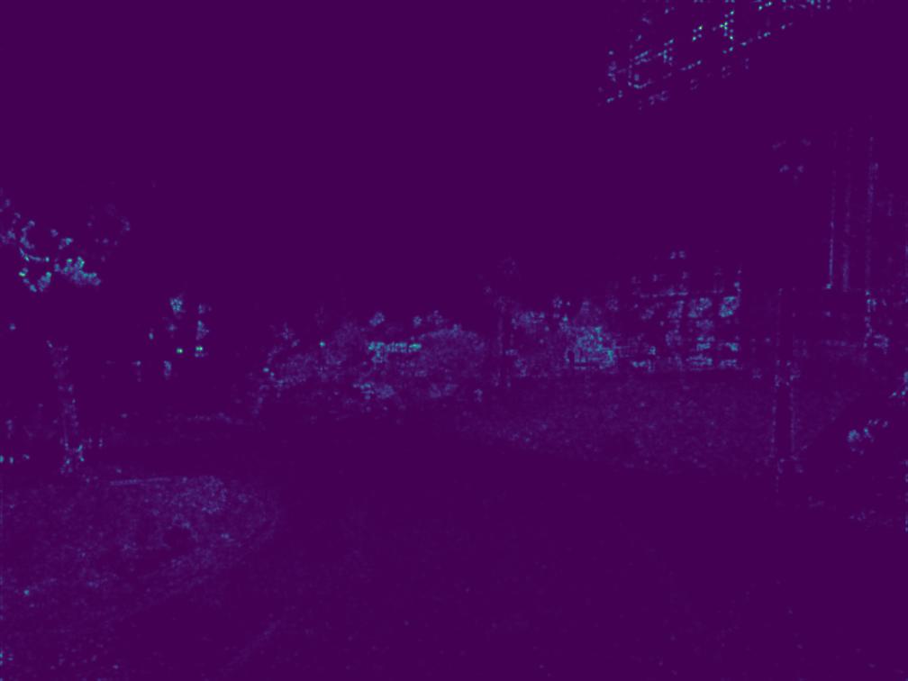
Path Left Harris Detector Results
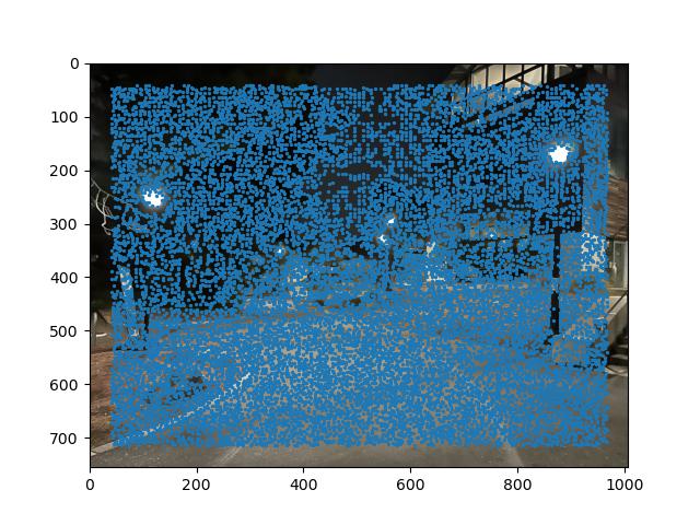
Path Left Points of Interest

Path Right Points of Interest
The sheer volume of points means some technique is needed to select an even distribution of the best ones to use that enables corresponding points to be found over a large section of the image without points doing the same thing or getting in each others way. ANMS finds radii around the points where they are the strongest, suppressing points that are significantly weaker points nearby and ensuring the remaining points are spread out around the image without being too close together.
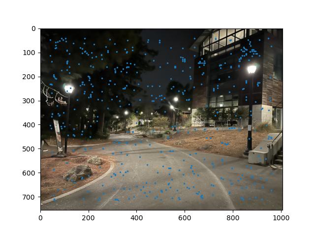
Path Left ANMS Results
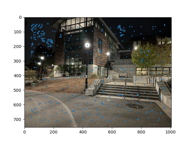
Path Right ANMS Results
To ensure the features at the remaining points left after ANMS is performed can be compared, descriptors of each feature had to be extracted. An 8 by 8 patch of pixels were extracted from an 80 by 80 pixel section of the image around each feature. Two examples of feature descriptors are shown below.

Path Left Feature Descriptor Example

Path Right Feature Descriptor Example
Features were matched using Lowe's approach, by finding the euclidean distance between the descriptors and finding the ratio of the euclidean distance of the nearest nearbor and the euclidean distance of the second nearest neighbor. Because points that are clearly corresponding would have a small ratio due to the second nearest neighbor likely being some random point much farther away, this allows for selecting the pairs most likely to be valid based on some threshold, and the outlier pairs that don't have valid corresponding points to be easily removed.

Path Left Corresponding Points
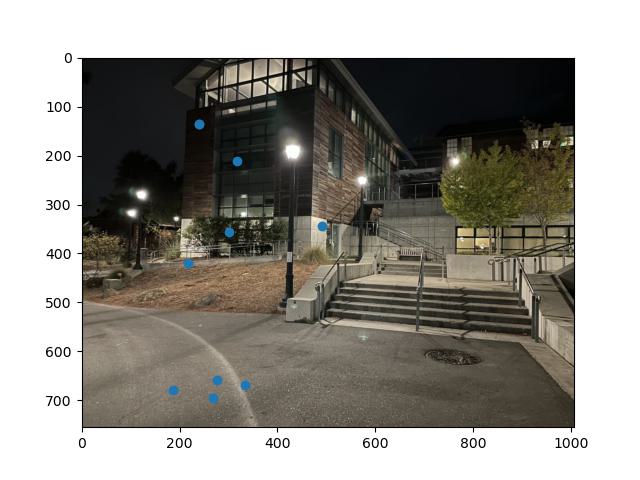
Path Right Corresponding Points
To finally select the best points to compute a homography with and compute that homography, 4-point RANSAC was used. Because there are still outliers even after using Lowe's trick, another method is needed to find and remove any last outliers, leaving the points that correspond with results that best warp the points of one image such that they match the other image. RANSAC works by randomly sampling 4 pairs of points from the points left after the previous step at a time and computing a homography. This homography is then used on all the valid points and the points that are within a threshold distance to their corresponding points are placed together in a set, without the outliers. This is repeated, and the largest set is saved to be used as it means the computed homography was accurate over the most points. The full set of these valid points were then used to compute the actual homographies used to warp the images. The results for the left image are below.
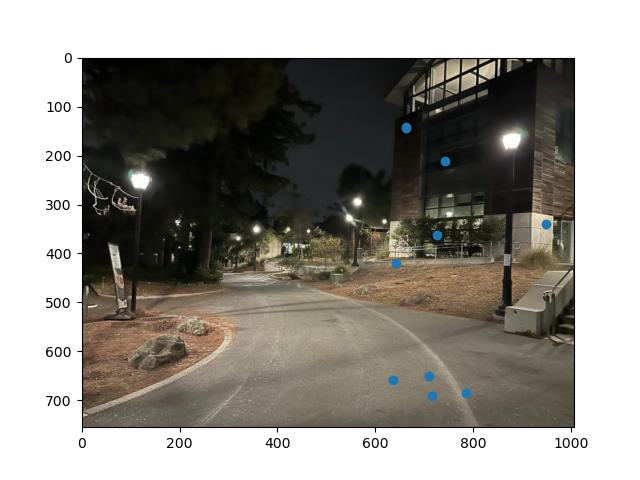
Path Left RANSAC Results
The results for the three pairs of images mosiaced and blended together are shown below. The path and dishrack images are shown alongside the results from manual selection of corresponding points. While the path images did very well at around the same as the manual matching, the dishrack was distinctly off and I was unable to obtain closer results from the selected points.
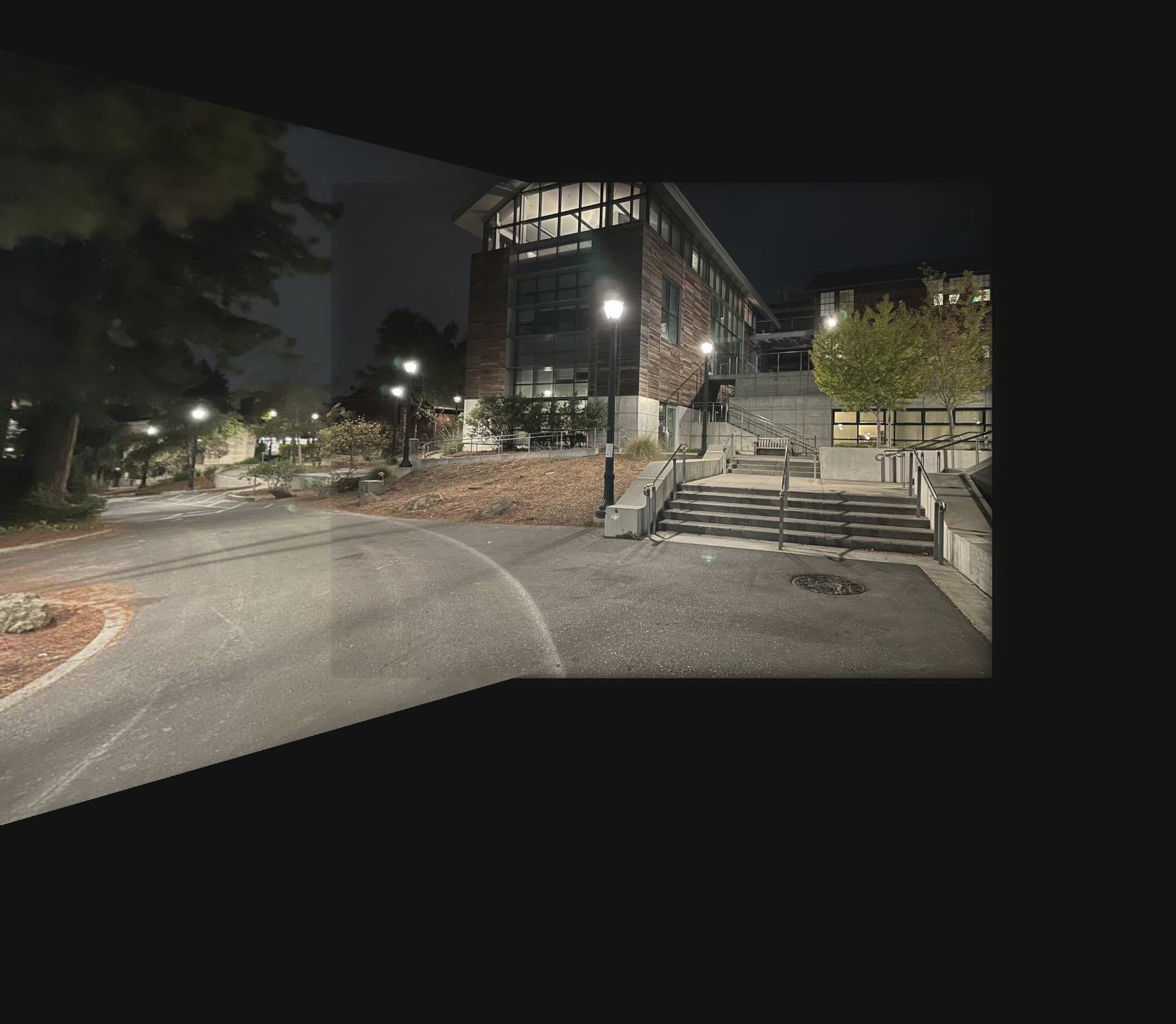
Path Left Autostitching Result

Path Left Original Result
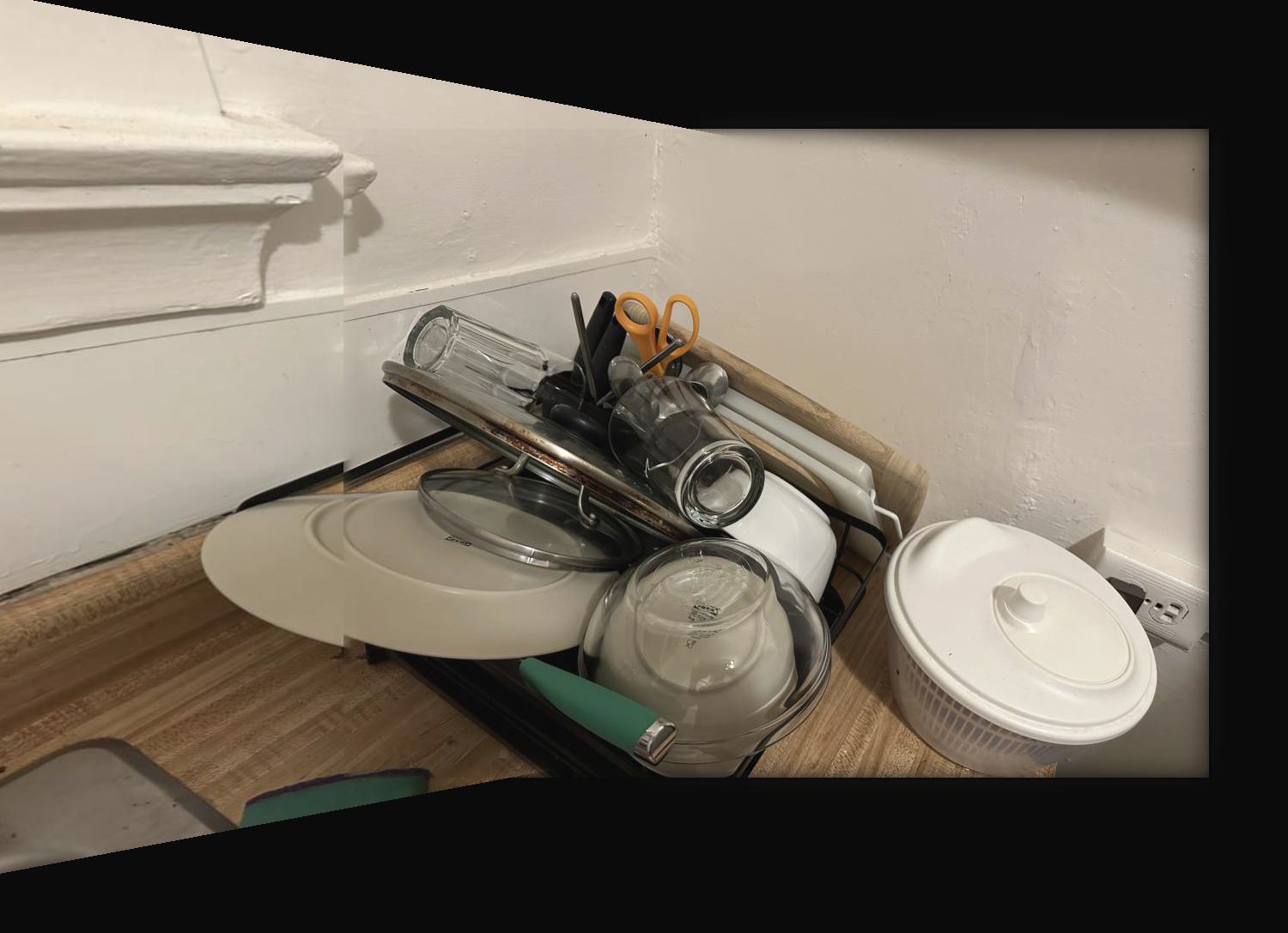
Dish Left Autostitching Result

Dish Left Original Result
I couldn't get the images for the split path to match at all, generally due to the little dots in the trees causing various detected corners to look far too similar to each other. For the third image, I took a new pair of images from my school club's (Pioneers in Engineering) room which actually autostitched together pretty well but with a slight visible distortion still.
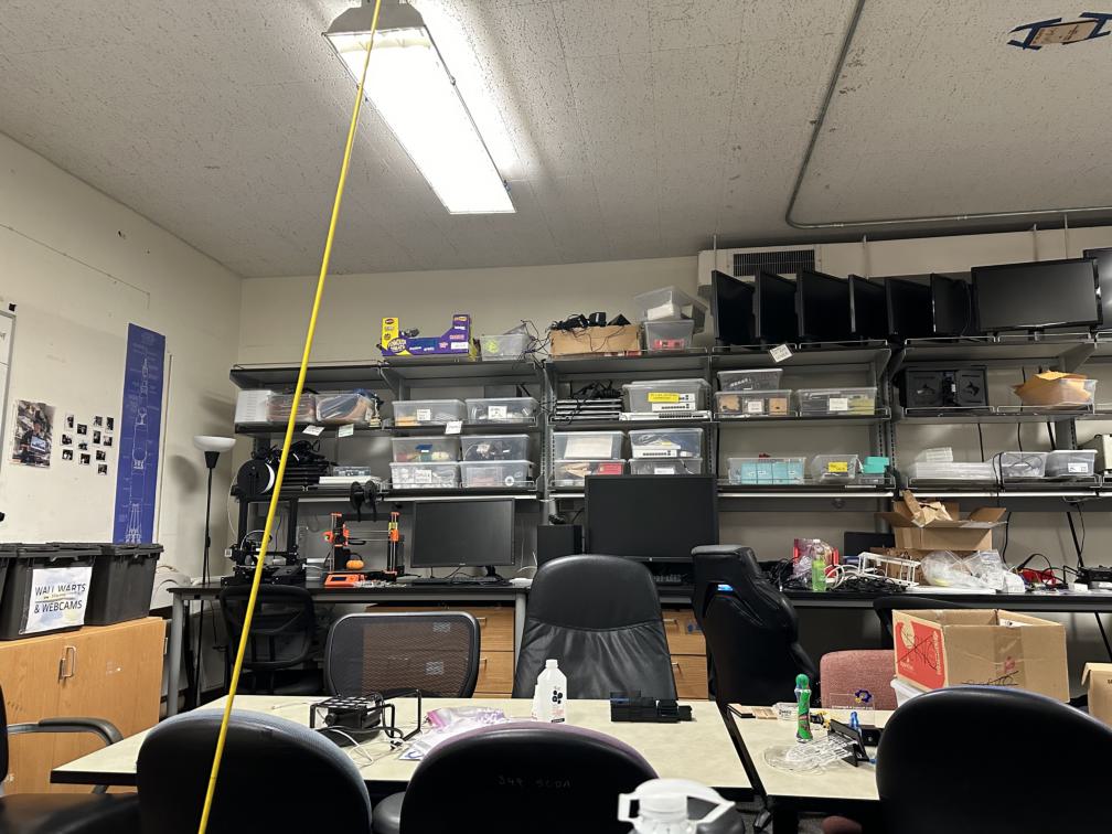
Student Club Room Left
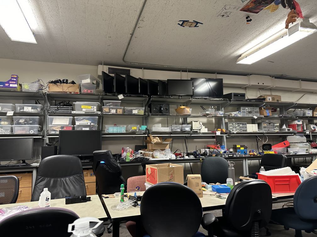
Student Club Room Right
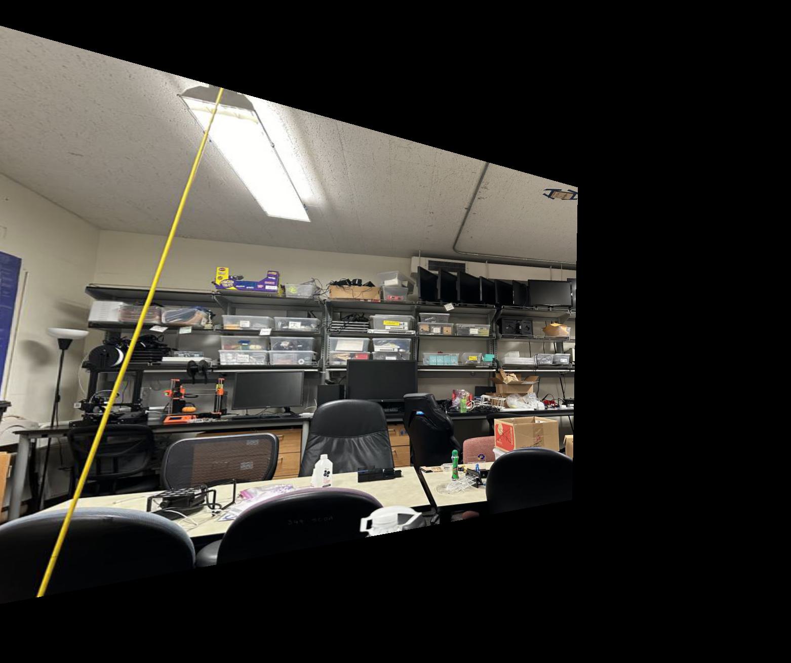
Student Club Room Left Warped
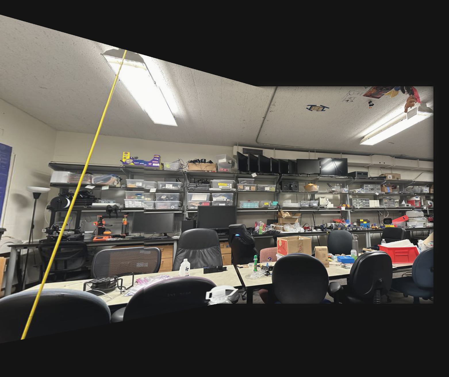
Student Club Room Autostitching Result
Automatic point detection has honestly been really cool to learn about and work on implementing. The several steps required that each do different things to shrink the number of possible corresponding points improve the next step have been really interesting; the fact that there is so much information that can be extracted and used from images to do things like figure out how they match has been really interesting to see in action.